brfss <- read.csv('C:/Users/15856/Downloads/Behavioral_Risk_Factor_Surveillance_System_(BRFSS)_Prevalence_Data_(2011_to_present)_20260428.csv')

paged_table(brfss)Exercise Patterns Across Income and Education Levels in the United States
DANL 310: Data Visualization and Presentation
Project Overview
Physical activity is an important part of overall health. However, not everyone exercises the same amount, which may be influenced by social and economic factors. This topic highlights how health behaviors are shaped by more than just personal preference. Factors such as income and education can affect an individual’s access to time, resources, and opportunities for physical activity. This may contribute to differences in exercise rates across groups. This project examines how exercise participation varies across income and education levels in the United States. The main question is: Are individuals with higher income and education more likely to engage in physical activity?
Data
The dataset used in this project is from the Behavioral Risk Factor Surveillance System (BRFSS), a national survey conducted by the Centers for Disease Control and Prevention (CDC). This survey collects self-reported information from adults in all 50 states on health behaviors and related factors. The data used in this project is from 2024. The unit of observation is a group defined by demographic categories, including income and education level. This analysis focuses on three main variables: exercise participation, income level, and education level. Exercise participation is measured as the percentage of individuals within each group who have engaged in physical activity in the past 30 days. Income and education are reported in categories. Although the data is self-reported, it still offers useful insights into health behavior across the United States.
Data Preparation and Transformation
To prepare for the analysis, the dataset was first filtered to include only respondents who had exercised in the past 30 days. It was also filtered to include the relevant demographic categories, including income and education. Observations with missing values were removed. Key variables such as exercise rates and sample sizes were converted to numeric format. The data was then grouped by income and education categories. A weighted average of exercise participation was calculated for each group using the sample size as weights. This ensures that groups with larger sample sizes have a greater influence on the results.
brfss_clean <- brfss |>
  filter(Response == "Yes") |>
  filter(Break_Out_Category %in% c("Household Income", "Education Attained"))

brfss_clean <- brfss_clean |>
  filter(!is.na(Data_value), !is.na(Sample_Size))

brfss_clean <- brfss_clean |>
  mutate(
    Data_value = as.numeric(Data_value),
    Sample_Size = as.numeric(gsub(",", "", Sample_Size))
  )

income_df <- brfss_clean |>
  filter(Break_Out_Category == "Household Income") |>
  group_by(Break_Out) |>
  summarize(
    exercise_rate = weighted.mean(Data_value, Sample_Size, na.rm = TRUE)
  ) |>
  rename(income = Break_Out)

income_df$income <- factor(income_df$income, levels = c(
  "Less than $15,000",
  "$15,000-$24,999",
  "$25,000-$34,999",
  "$35,000-$49,999",
  "$50,000-$99,999",
  "$100,000-$199,999",
  "$200,000+"
))

income_df <- income_df |>
  filter(!is.na(income))

education_df <- brfss_clean |>
  filter(Break_Out_Category == "Education Attained") |>
  group_by(Break_Out) |>
  summarize(
    exercise_rate = weighted.mean(Data_value, Sample_Size, na.rm = TRUE)
  ) |>
  rename(education = Break_Out)

education_df$education <- factor(education_df$education, levels = c(
  "Less than H.S.",
  "H.S. or G.E.D.",
  "Some post-H.S.",
  "College graduate"
))
Descriptive Statistics
Basic Summary
skim(brfss_clean)| Name | brfss_clean |
| Number of rows | 7095 |
| Number of columns | 10 |
| _______________________ | |
| Column type frequency: | |
| character | 5 |
| numeric | 5 |
| ________________________ | |
| Group variables | None |
Variable type: character
| skim_variable | n_missing | complete_rate | min | max | empty | n_unique | whitespace |
|---|---|---|---|---|---|---|---|
| Locationabbr | 0 | 1 | 2 | 2 | 0 | 54 | 0 |
| Locationdesc | 0 | 1 | 4 | 20 | 0 | 54 | 0 |
| Response | 0 | 1 | 3 | 3 | 0 | 1 | 0 |
| Break_Out | 0 | 1 | 8 | 17 | 0 | 12 | 0 |
| Break_Out_Category | 0 | 1 | 16 | 18 | 0 | 2 | 0 |
Variable type: numeric
| skim_variable | n_missing | complete_rate | mean | sd | p0 | p25 | p50 | p75 | p100 | hist |
|---|---|---|---|---|---|---|---|---|---|---|
| Year | 0 | 1 | 2017.79 | 4.09 | 2011.0 | 2014.0 | 2018.0 | 2021.0 | 2024.0 | ▆▆▅▇▇ |
| Sample_Size | 0 | 1 | 1191.99 | 1240.17 | 44.0 | 380.0 | 775.0 | 1570.0 | 16152.0 | ▇▁▁▁▁ |
| Data_value | 0 | 1 | 72.64 | 10.64 | 33.2 | 64.9 | 72.5 | 80.9 | 97.4 | ▁▂▇▇▃ |
| Confidence_limit_Low | 0 | 1 | 68.59 | 12.10 | 28.2 | 59.7 | 68.5 | 78.2 | 96.0 | ▁▃▇▇▃ |
| Confidence_limit_High | 0 | 1 | 76.68 | 9.51 | 37.3 | 69.9 | 76.7 | 83.7 | 100.0 | ▁▁▇▇▃ |
Important Statistics
Exercise rate:
# overall exercise rate
overall_exercise <- weighted.mean(
  brfss_clean$Data_value,
  brfss_clean$Sample_Size,
  na.rm = TRUE
)

overall_exercise
[1] 78.2776Income groups range:
range(income_df$exercise_rate, na.rm = TRUE)[1] 61.94568 92.31137Education groups range:
range(education_df$exercise_rate, na.rm = TRUE)[1] 58.64922 86.85935The descriptive statistics show clear variation across socioeconomic groups. The overall average exercise rate is about 78%. Income groups range from about 62% to 92%, whereas education groups range from about 59% to 87%. The differences within groups are slightly more pronounced across income levels, suggesting larger gaps by income.
Data Visualization
Visualization 1: Exercise Rates by Income
ggplot(income_df, aes(x = income, y = exercise_rate)) +
  geom_col(fill = "#4E79A7") +
  labs(
    title = "Exercise Rates by Income",
    x = "Income Level",
    y = "Exercise Rate (%)"
  ) +
  theme_minimal(base_size = 14) +
  theme(
    plot.title = element_text(face = "bold", size = 16),
    axis.text.x = element_text(angle = 45, hjust = 1),
    panel.grid.minor = element_blank()
  )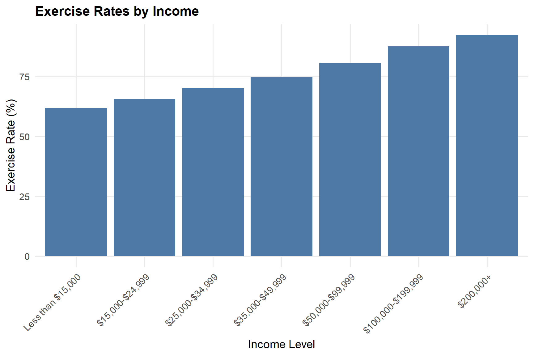
This chart shows a clear positive relationship between income and exercise rates. As income increases, the percentage of individuals who report exercising in the past 30 days also increases. This pattern suggests that higher income individuals are more likely to participate in physical activity. This could be because having a higher income provides greater access to resources that support exercise, such as gym memberships, safe neighborhoods, and flexible time. These resources may be less available to lower income groups.
Visualization 2: Exercise Rates by Education
ggplot(education_df, aes(x = education, y = exercise_rate)) +
  geom_col(fill = "#59A14F") +
  labs(
    title = "Exercise Rates by Education",
    x = "Education Level",
    y = "Exercise Rate (%)"
  ) +
  theme_minimal(base_size = 14) +
  theme(
    plot.title = element_text(face = "bold"),
    axis.text.x = element_text(angle = 45, hjust = 1),
    panel.grid.minor = element_blank()
  )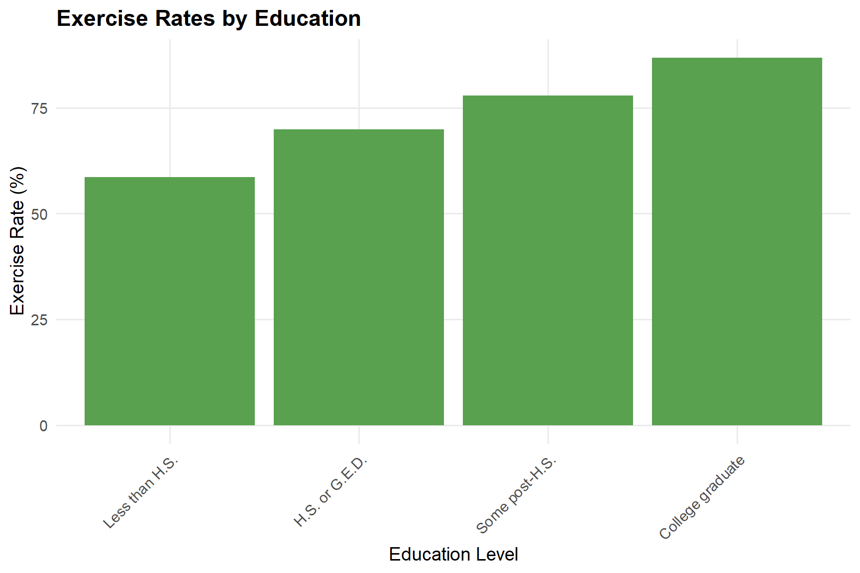
This chart shows a similar positive relationship between education level and exercise rates. Individuals with less than a high school edcuation have the lowest exercise rate (about 60%), whereas college graduates have the highest exercise rate (about 90%). Each step up in education level is correlated with an increase in exercise participation. This suggests that education is strongly associated with healthier behaviors like exercise. Higher levels of education may increase awareness of the benefits of physical activity and correlate with occupations that give an individual more time or opportunity to exercise.
Visualization 3: Exercise Rates Across United States
ggplot(map_df, aes(long, lat, group = group, fill = exercise_rate)) +
  geom_polygon(color = "white", size = 0.2) +
  coord_fixed(1.3) +
  scale_fill_gradient(low = "#DEEBF7", high = "#3182BD", na.value = "grey90") +
  labs(
    title = "Exercise Rates Across United States",
    fill = "Exercise Rate (%)"
  ) +
  theme_void() +
  theme(
    plot.title = element_text(face = "bold", size = 16),
    legend.position = "right"
  )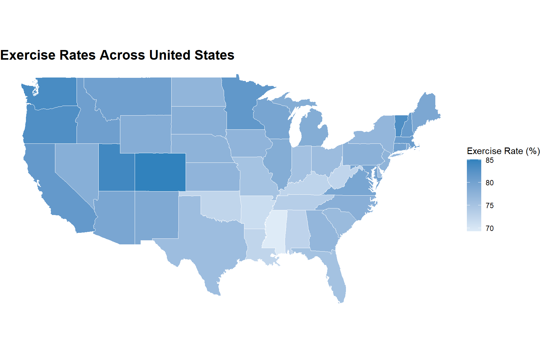
This map shows geographic variation in exercise rates across states. Some states show much higher levels of physical activity than others. Western and a few northeastern states tend to have higher exercise rates (darker shades), while some southern and midwestern states appear to have lower rates (lighter shades). These regional differences may reflect socioeconomic and environmental factors, such as differences in income distribution, education levels, climate, and infrastructure.
Shiny App
This Shiny application provides an interactive exploration of exercise rates by income and education. The app allows the user to view and compare the first two visualizations of this project dynamically. This app aims to help examine how health behaviors, like exercise, vary across socioeconomic groups.
Dashboard
- Dashboard: View Dashboard
This dashboard explores how exercise rates vary by income, education, geography across the United States. It allows the user to compare differences in physical activity across socioeconomic groups and states, helping to identify patterns in health behavior.
Discussion
The visualizations suggest that exercise rates increase with both income and education. People with higher income and education levels tend to report higher rates of physical activity. One possible explanation is they have greater access to resources such as gym memberships, safe places to exercise, and more free time. Overall, these patterns show that exercise rates follow a social and economic pattern. The geographic results also show variation across states. This suggests that location and environment may also affect physical activity.
Limitations
This analysis is purely descriptive, meaning it does not show causal relationships. Although the visualizations show relationships between income, education, and exercise rates, they do not prove that one variable causes another.
There are also limitations in the data itself. Exercise rates are self reported, which may not be completely accurate. Additionally, some observations are missing, which may impact the accuracy of the geographic visualization.
Finally, other important factors like age and health status are not included in this analysis, which may also influence exercise behavior.
Conclusion
This project explores how exercise rates differ by income, education, and geography. The results show a clear pattern: people with higher income and education tend to exercise more, with variation across states. Overall, the results suggest that exercise is influenced by social and economic factors, not just personal preference. Access to resources and opportunity appear to play an important role in health behaviors.
Future Directions
Future work could include additional variables such as age, occupation, or health status. This would help provide a more complete understanding of what influences physical activity. It would also be useful to examine a longer period of time to see whether these patterns change over time. More detailed geographic analysis at the county level could also provide a clearer picture of variation across and within regions. Finally, this project could include more advanced modeling approaches to isolate the effects of different socioeconomic factors and analyze correlations between variables.
References
Centers for Disease Control and Prevention (CDC). (n.d.). Behavioral Risk Factor Surveillance System (BRFSS). https://www.cdc.gov/brfss/ (Accessed May 2026).
R Core Team. (2024). R: A language and environment for statistical computing. https://www.r-project.org/ (Accessed May 2026).
Wickham, H. et al. (2019). tidyverse: Easily install and load the tidyverse. https://www.tidyverse.org/ (Accessed May 2026).
Wickham, H. ggplot2: Create elegant data visualisations. https://ggplot2.tidyverse.org/ (Accessed May 2026).
Wickham, H. dplyr: A grammar of data manipulation. https://dplyr.tidyverse.org/ (Accessed May 2026).
Pebesma, E. sf: Simple features for R. https://r-spatial.github.io/sf/ (Accessed May 2026).
Ahlmann-Eltze, C. skimr: Compact and flexible summaries of data. https://docs.ropensci.org/skimr/ (Accessed May 2026).
RStudio. rmarkdown: Dynamic documents for R. https://rmarkdown.rstudio.com/ (Accessed May 2026).
Cédric Scherer. hrbrthemes: Additional themes for ggplot2. https://github.com/hrbrmstr/hrbrthemes (Accessed May 2026).
R Core / R community. maps: Draw geographical maps. https://cran.r-project.org/package=maps (Accessed May 2026).
Posit. shiny: Web application framework for R. https://shiny.posit.co/ (Accessed May 2026).
OpenAI. (2026). ChatGPT (GPT-5.3). https://chat.openai.com/ (Accessed May 2026).