path <- 'https://bcdanl.github.io/data/climate_finance_energy.csv'
climate_finance <- read_csv(path)DANL Project
Climate Finance
1 Introduction
About this project 👏
This project will address the various financial actions taken by various parties to address climate change.
2 Data
2.1 Variable Description
Party: a party (country) that provides a funding contribution to recipient country/region for their cliamte change project.
Recipient country/region: Recipient country or region
Project/programme/activity: Details in the climate change project
Type of support:
adaptation if the climate change project is related to adaptation project.
mitigation if the climate change project is related to mitigation project.
Year: Year that funding contribution is committed or provided.
Contribution: An amount of funding contribution for the climate change project (in USD).
Status:
committed if a party commits to providing the funding contribution for the climate change project, but the funding contribution is NOT actually provided.
provided if the funding contribution was provided for the climate change project.
Energy:
TRUE if the project is energy-related;
FALSE otherwise.
2.2 Summary Statistics
skim(climate_finance) %>%
select(-n_missing)| Name | climate_finance |
| Number of rows | 16853 |
| Number of columns | 8 |
| _______________________ | |
| Column type frequency: | |
| character | 5 |
| logical | 1 |
| numeric | 2 |
| ________________________ | |
| Group variables | None |
Variable type: character
| skim_variable | complete_rate | min | max | empty | n_unique | whitespace |
|---|---|---|---|---|---|---|
| Party | 1.00 | 5 | 24 | 0 | 34 | 0 |
| Recipient country/region | 1.00 | 3 | 293 | 0 | 1310 | 0 |
| Project/programme/activity | 0.68 | 3 | 1473 | 0 | 7908 | 0 |
| Type of support | 1.00 | 10 | 10 | 0 | 2 | 0 |
| Status | 1.00 | 8 | 9 | 0 | 2 | 0 |
Variable type: logical
| skim_variable | complete_rate | mean | count |
|---|---|---|---|
| Energy | 1 | 0.19 | FAL: 13710, TRU: 3143 |
Variable type: numeric
| skim_variable | complete_rate | mean | sd | p0 | p25 | p50 | p75 | p100 | hist |
|---|---|---|---|---|---|---|---|---|---|
| Year | 1 | 2015.72 | 1.82 | 2011 | 2015 | 2016 | 2017 | 2018 | ▁▂▆▅▇ |
| Contribution | 1 | 3311433.39 | 9714907.28 | 3000 | 100000 | 420000 | 2200000 | 100000000 | ▇▁▁▁▁ |
3 Analysis
3.1 Financial Contributions to Other Countries
Various parties in the climate_finance data frame have made positive financial contributions to other countries for adaptation projects. Here, we will find the number of parties that made a positive contribution to another country for every year between 2011 and 2018.
positive_contributions <- climate_finance %>%
  filter(Status == "provided",
         `Type of support` == "adaptation") %>%
  group_by(Party, Year) %>%
  summarise(Contribution = sum(Contribution, na.rm = T)) %>%
  filter(Contribution > 0) %>%
  group_by(Party) %>%
  count() %>%
  filter(n == 2018 - 2011 + 1)  %>%
  select(Party) %>%
distinct() nrow(positive_contributions)[1] 83.2 Types of Contributions
There are two different types of contributions that a party can make: adaptation and mitigation. The type of contribution is decided based on the type of project it supports. Adaptation contributions go to an adaptation climate change project. A mitigation contribution goes to a mitigation climate change project.
First, we will calculate the ratio between adaptation contribution and mitigation contribution for each type of Status for each Party each year.
ratio <- climate_finance %>%
  group_by(Party, Year, Status, `Type of support`) %>%
  summarise(Contribution = sum(Contribution, na.rm = T)) %>%
  filter(Contribution != 0) %>%
  group_by(Party, Year, Status) %>%
  mutate(lag_Contribution = lag(Contribution),
         am_ratio = lag_Contribution / Contribution ) %>%
  filter(!is.na(am_ratio)) %>%
  rename(mitigation = Contribution,
         adaptation = lag_Contribution) %>%
  select(-`Type of support`)
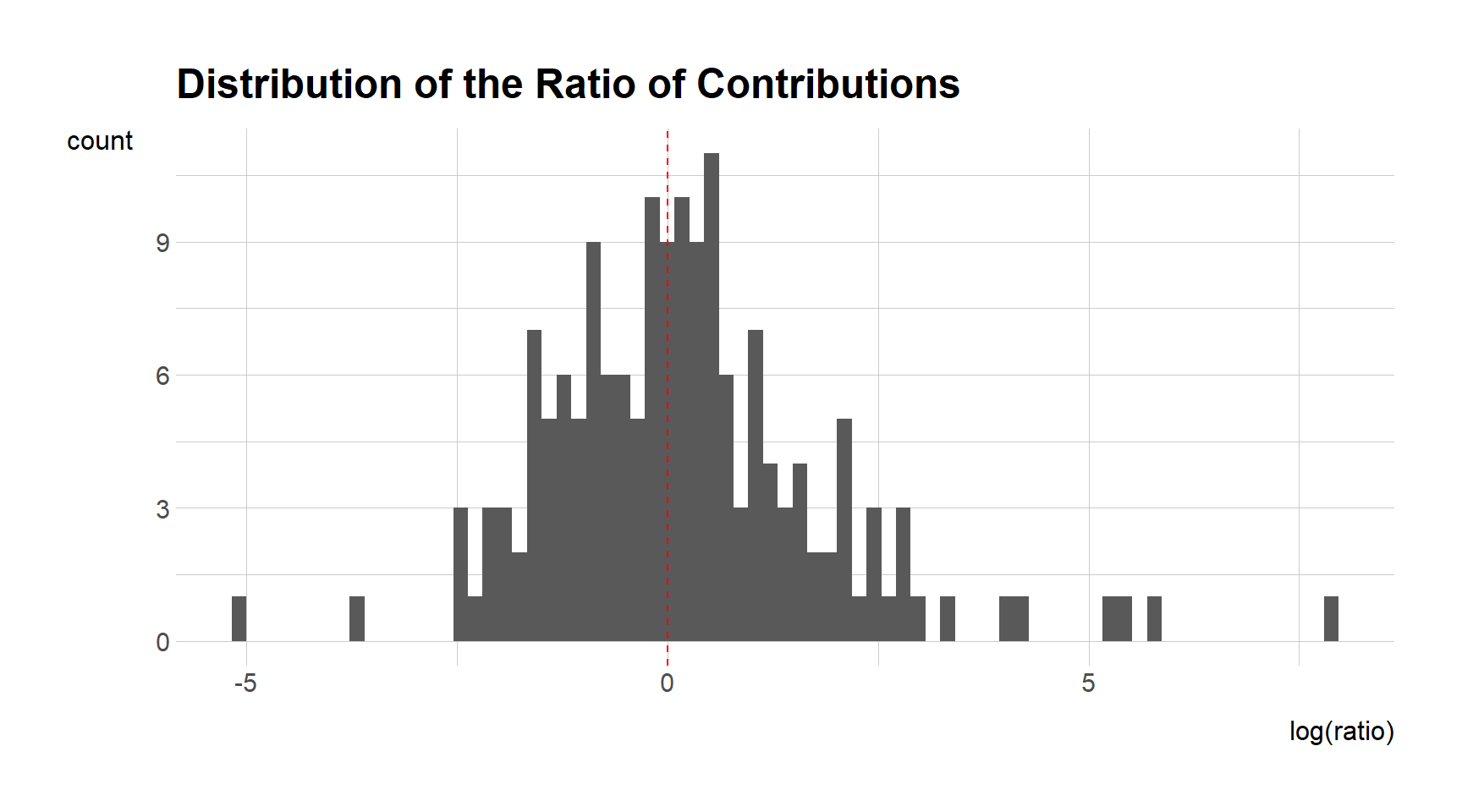
Here, we will visualize the distribution of the ratio between adaption contribution and mitigation contribution based on our calculation.
ggplot(ratio, aes(x = log(am_ratio))) +
  geom_histogram(bins = 75) + labs(x = "log(ratio)", y = "count", title = "Distribution of the Ratio of Contributions") +
  geom_vline(xintercept = 0, color = 'red', lty = 2)
This histogram depicts a generally normal distribution of the ratio between adaptation contribution and mitigation contribution.
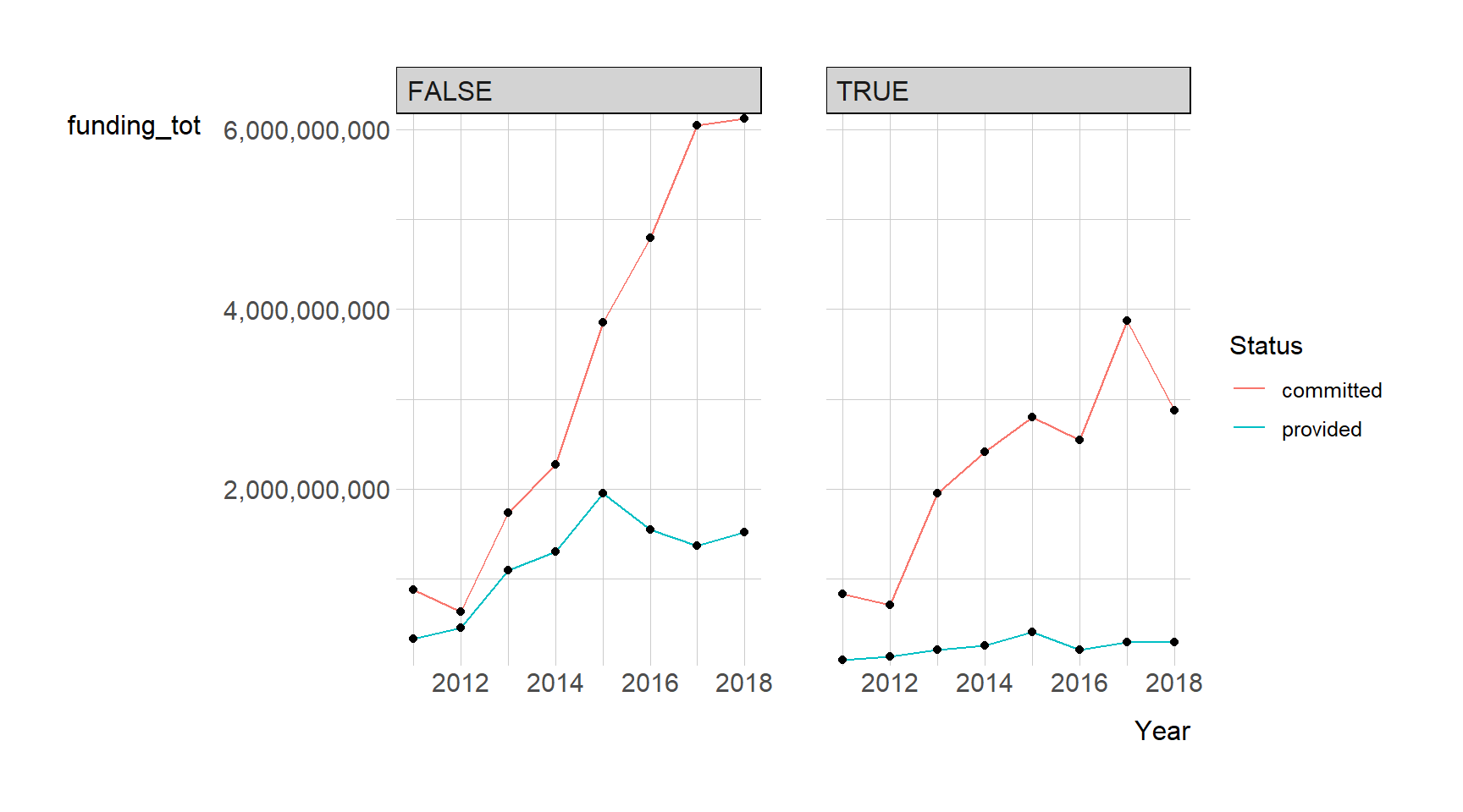
3.3 Yearly trend of total funding contributions varies by Energy and Status
With these graphs we can see the amount of committed funding has been increasing at a significant rate while provided funding seems to stay constant. The gap we see in provided funding size between the energy and non energy sectors is likely due to these projects requiring a significant amount of funds upfront.
climate_finance %>%
  group_by(Energy, Status, Year) %>%
  summarise(funding_tot = sum(Contribution, na.rm = T)) %>%
  ggplot(aes(x = Year, y = funding_tot)) +
  geom_line(aes(color = Status)) +
  geom_point() +
  facet_wrap(Energy ~.) +
  scale_y_comma()
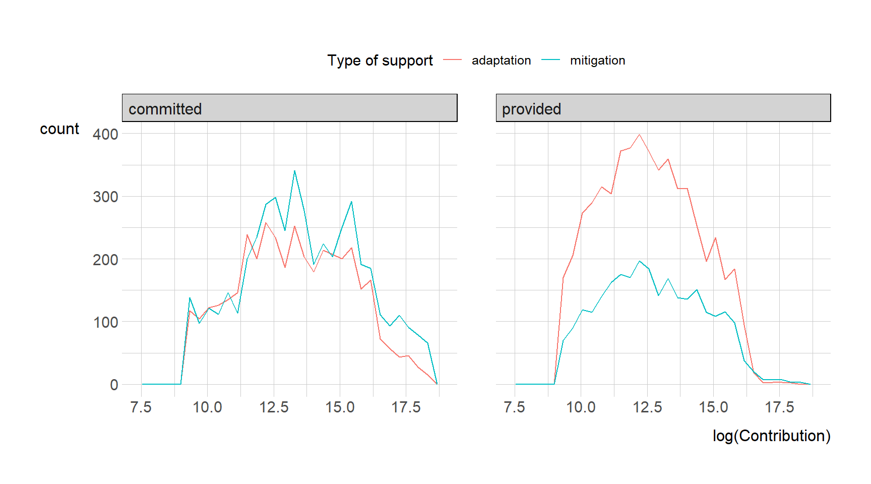
3.4 Yearly Contribution varying by Energy and Status
For both sectors (energy and non-energy), the amount of the committed funding has been increasing yearly, while the amount of provided funding has stayed relatively constant. Energy related projects usually require a much greater upfront cost than non-energy related projects, hence why there is a gap for the provided amounts.
ggplot(climate_finance,
       aes(color = `Type of support`, x = log(Contribution))) +
  geom_freqpoly() +
  facet_wrap(.~ Status) +
  theme(legend.position = 'top')
4 Summary
There is not one set path or action to take to solve the climate change crisis, as demonstrated by the various amounts and types of funding actions. Climate finance is a complicated subject, but to solve the problem, more action (such as actually providing funds instead of just committing to it) is needed by all parties.