Beer Markets

Let’s analyze the beer_mkts data:

beer_mkts <- read_csv("https://bcdanl.github.io/data/beer_markets.csv")

rmarkdown::paged_table(beer_mkts) 

Variable Description for beer_mkts data.frame

The following describes the variables in the beer_mkts data.frame.

• hh: Household identifier
• _purchase_desc: Description of the purchase
• quantity: The quantity of beer purchased
• brand: The brand of beer
• dollar_spent: The amount spent
• beer_floz: Fluid ounces of beer
• price_per_floz: Price per fluid ounce
• container: Type of container
• promo: Whether the purchase was on promotion
• market: The market where the purchase was made
• Demographics: age, employment status, degree, class of worker (cow), race, and household information like microwave, dishwasher, tvcable, singlefamilyhome, and npeople (number of people in the household)

Purchase Patterns

We’ll explore the purchase patterns for beer purchases in the dataset. This will include finding the most popular brands and spending habits across different markets. Here are some specific analyses we can perform:

• Find top markets in terms of total quantity for each brand.

• Compare the proportion of loyal customers.

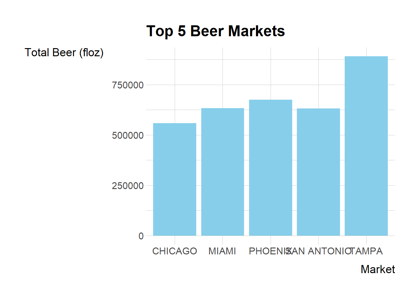
I’ll begin with these analyses and create visualizations to help us understand the data better. I will start by finding the top 5 markets in terms of the total beer_floz.

top_5 <- beer_mkts %>% 
   group_by(market) %>% 
   summarize(beer_floz_tot = sum(beer_floz, na.rm = T)) %>% 
   arrange(-beer_floz_tot) %>% 
   slice(1:5)

Let’s visualize the top 5 markets in terms of the total beer_floz.

ggplot(top_5, aes(x = market, y = beer_floz_tot)) +
  geom_bar(stat = "identity", fill = "skyblue") +
  labs(title = "Top 5 Beer Markets",
       x = "Market",
       y = "Total Beer (floz)")

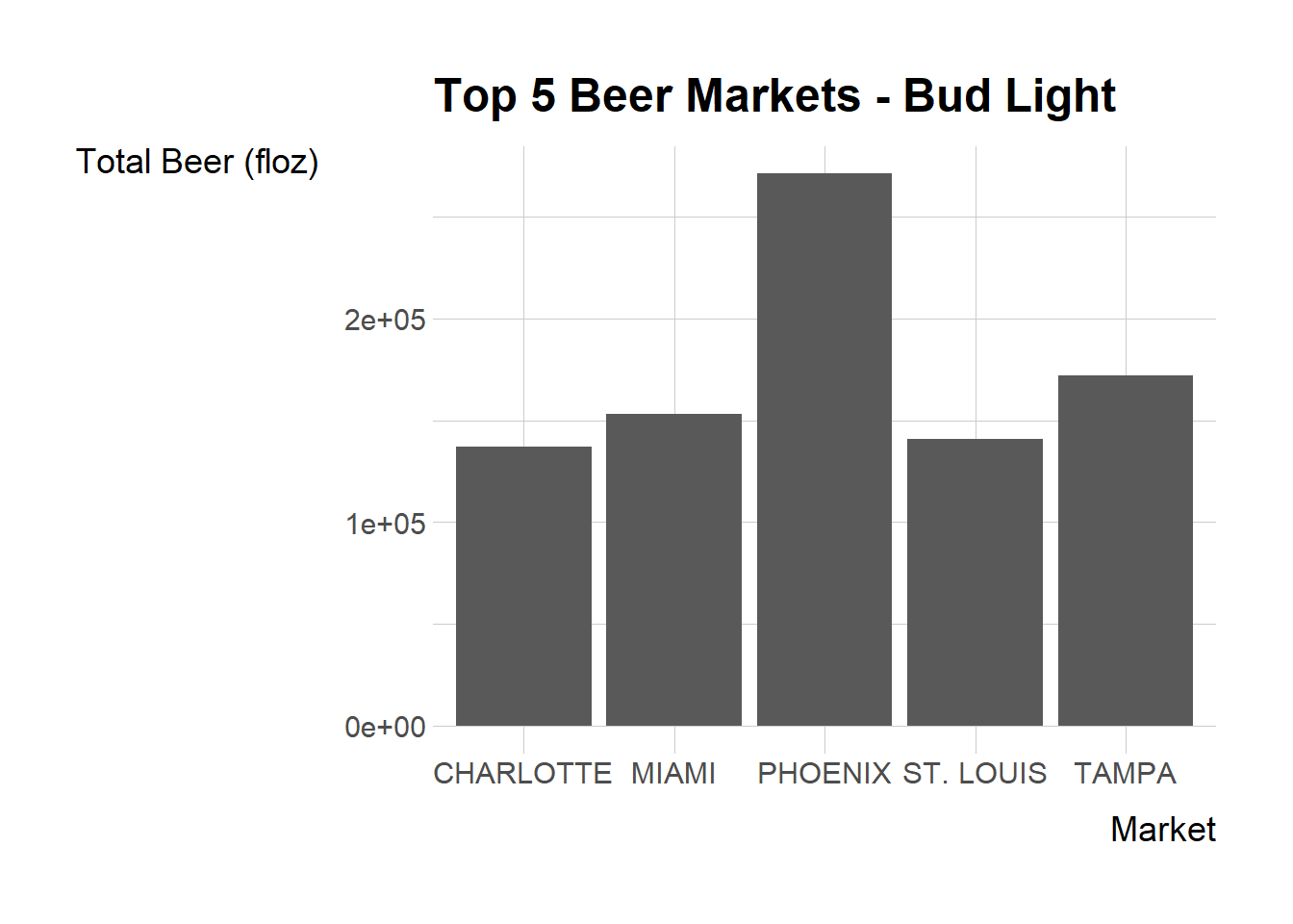
Next, we can look at the top 5 markets in terms of the total beer_floz of a specific brand. For example, BUD LIGHT:

top_5_bud <- beer_mkts %>% 
  filter(brand == "BUD LIGHT") %>% 
  group_by(market) %>% 
  summarize(beer_floz_tot = sum(beer_floz, na.rm = T)) %>% 
  arrange(-beer_floz_tot) %>% 
  slice(1:5)

Just like the top 5 beer markets, let’s visualize the top 5 markets for BUD LIGHT.

ggplot(top_5_bud, aes(x = market, y = beer_floz_tot)) +
  geom_bar(stat = "identity") +
  labs(title = "Top 5 Beer Markets - Bud Light",
       x = "Market",
       y = "Total Beer (floz)")

I will do the same for BUSCH LIGHT, COORS LIGHT, MILLER LITE, and NATURAL LIGHT.

top_5_busch <- beer_mkts %>% 
  filter(brand == "BUSCH LIGHT") %>% 
  group_by(market) %>% 
  summarize(beer_floz_tot = sum(beer_floz, na.rm = T)) %>% 
  arrange(-beer_floz_tot) %>% 
  slice(1:5)

top_5_coors <- beer_mkts %>% 
  filter(brand == "COORS LIGHT") %>% 
  group_by(market) %>% 
  summarize(beer_floz_tot = sum(beer_floz, na.rm = T)) %>% 
  arrange(-beer_floz_tot) %>% 
  slice(1:5)

top_5_miller <- beer_mkts %>% 
  filter(brand == "MILLER LITE") %>% 
  group_by(market) %>% 
  summarize(beer_floz_tot = sum(beer_floz, na.rm = T)) %>% 
  arrange(-beer_floz_tot) %>% 
  slice(1:5)

top_5_natural <- beer_mkts %>% 
  filter(brand == "NATURAL LIGHT") %>% 
  group_by(market) %>% 
  summarize(beer_floz_tot = sum(beer_floz, na.rm = T)) %>% 
  arrange(-beer_floz_tot) %>% 
  slice(1:5)

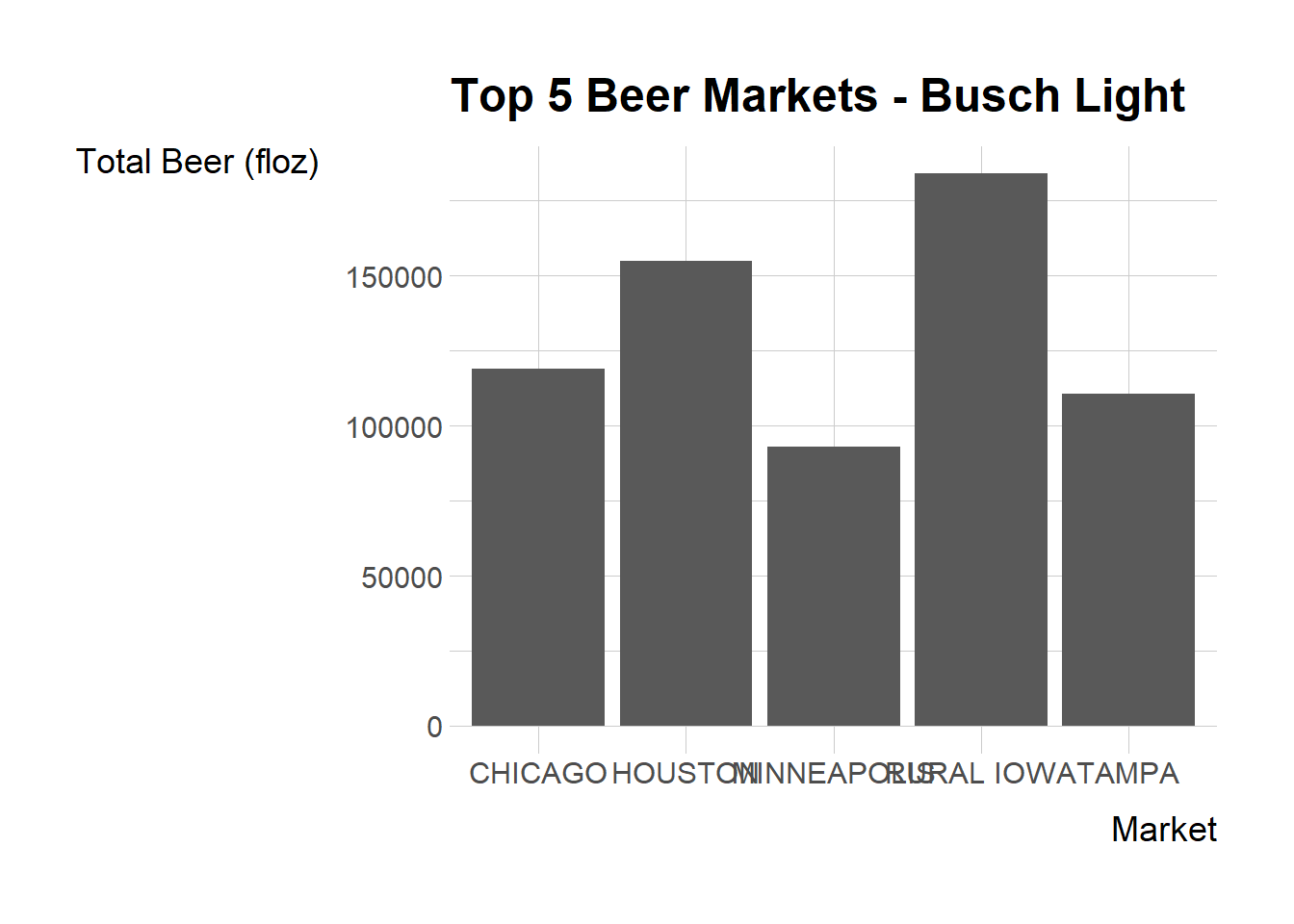
Let’s also look at a visualization for BUSCH LIGHT:

ggplot(top_5_busch, aes(x = market, y = beer_floz_tot)) +
  geom_bar(stat = "identity") +
  labs(title = "Top 5 Beer Markets - Busch Light",
       x = "Market",
       y = "Total Beer (floz)")

Next, we will evaluate proportions of loyal customers for each brand. For example, for households that purchased BUD LIGHT at least once, I will find the fraction of households that purchased only BUD LIGHT. I will find the proportion of loyal customers for all 5 brands.

loyal_customers <- beer_mkts %>% 
  mutate(bud = ifelse(brand=="BUD LIGHT", 1, 0), # 1 if brand=="BUD LIGHT"; 0 otherwise
         busch = ifelse(brand=="BUSCH LIGHT", 1, 0),
         coors = ifelse(brand=="COORS LIGHT", 1, 0),
         miller = ifelse(brand=="MILLER LITE", 1, 0),
         natural = ifelse(brand=="NATURAL LIGHT", 1, 0),
         .after = hh) %>% 
  select(hh:natural) %>%  # select the variables we need
  group_by(hh) %>% 
  summarise(n_transactions = n(), # number of beer transactions for each hh
            n_bud = sum(bud), # number of BUD LIGHT transactions for each hh
            n_busch = sum(busch), 
            n_coors = sum(coors), 
            n_miller = sum(miller), 
            n_natural = sum(natural) 
  ) %>% 
  summarise(loyal_bud = sum(n_transactions == n_bud) / sum(n_bud > 0), 
              # sum(n_transactions == n_bud) : the number of households that purchased BUD LIGHT only
              # sum(n_bud > 0) : the number of households that purchased BUD LIGHT at least once.
            loyal_busch = sum(n_transactions == n_busch) / sum(n_busch > 0),
            loyal_coors = sum(n_transactions == n_coors) / sum(n_coors > 0),
            loyal_miller = sum(n_transactions == n_miller) / sum(n_miller > 0),
            loyal_natural = sum(n_transactions == n_natural) / sum(n_natural > 0)
  )